Recently, we were doing some experiments with a SQL query that joins a few dimensional tables to enrich incoming records. While doing so, we were thinking of whether an implementation of the same task using the DataStream API would actually be able to squeeze some more performance out of the available machines. We would like to take you on this journey to see whether and how this is possible. We will also provide further hints for jobs that differ from our proof of concept (PoC) code and will present an outlook of the things to come.
SQL Query
First off, let us have a look at the query we are trying to outperform. The query outlined below is inspired from a real streaming SQL job we were given. It performs a join of an input stream from fact_table with a few dimensional tables defined as follows (with the data inside the dimensional tables as random strings of up to 100 characters each):

The important part of this job is that all input tables are subject to change; they are consumed as streams. In that case, we need to decide what version of a row to join with. This is where Flink’s temporal table joins come into place: each row from fact_table should be joined and merged with with the most recent row from the appropriate dimension tables at the time the join is executed. If you look further into temporal joins (via the LATERAL TABLE statement and a wrapping temporal table function around tables dim_table1, …, dim_table5), you will also see event-time join support which may come in handy. However, we are not using it here for simplicity.
SELECT
 D1.col1 AS A,
 D1.col2 AS B,
 D1.col3 AS C,
 D1.col4 AS D,
 D1.col5 AS E,
 D2.col1 AS F,
 D2.col2 AS G,
 ...
 D5.col4 AS X,
 D5.col5 AS Y
FROM
 fact_table,
 LATERAL TABLE (dimension_table1(f_proctime)) AS D1,
 LATERAL TABLE (dimension_table2(f_proctime)) AS D2,
 LATERAL TABLE (dimension_table3(f_proctime)) AS D3,
 LATERAL TABLE (dimension_table4(f_proctime)) AS D4,
 LATERAL TABLE (dimension_table5(f_proctime)) AS D5
WHERE
 fact_table.dim1  = D1.id
 AND fact_table.dim2 = D2.id
 AND fact_table.dim3 = D3.id
 AND fact_table.dim4 = D4.id
 AND fact_table.dim5 = D5.id
myThe surrounding DataStream code in LateralTableJoin.java creates a streaming source for each of the input tables and converts the output into an append DataStream that is piped into a DiscardingSink. There are two ways of setting up this SQL job in Flink 1.10: using the old Flink planner or using the new Blink planner. Let’s see what the differences are.
Old/Flink Planner
The old planner is currently (as of Flink 1.10) used by default or can be set manually via
StreamExecutionEnvironment env = StreamExecutionEnvironment.getExecutionEnvironment();
StreamTableEnvironment tEnv = StreamTableEnvironment
 .create(env, EnvironmentSettings.newInstance().useOldPlanner().build());
It will transform the SQL query to the following job graph with a few chained operations for transforming the DataStream sources to tables and creating the selected subset of columns after each join:
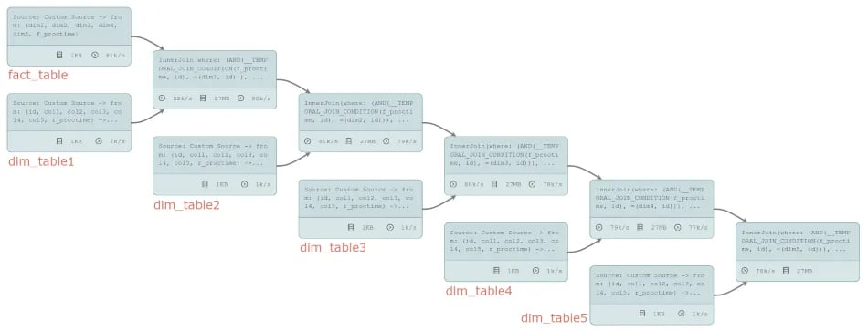
Out of the box, this gives a stable throughput of 84,279 events per second.
New/Blink Planner
Flink’s new Blink planner implements several enhancements such as an improved feature set and, when looking at performance, is working with binary types as much as possible to avoid serialization/deserialization overhead. It can be enabled during the initialization of the StreamTableEnvironment:
StreamExecutionEnvironment env = StreamExecutionEnvironment.getExecutionEnvironment();
StreamTableEnvironment tEnv = StreamTableEnvironment
 .create(env, EnvironmentSettings.newInstance().useBlinkPlanner().build());
The created job graph does not look too much different from the old planner and has similar conceptual operators:
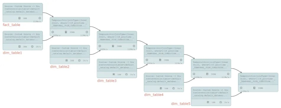
Simply enabling the Blink planner in this scenario increases throughput slightly to 89,048 events per second (+5%).
Object Reuse
Both planners create tasks that actually consist of two chained operations: the sources have some sort of table conversion / field selection appended, the (temporal) joins are followed by a selection of the fields as well. If you recall how Flink is handling the exchange of data objects between operators, you will notice that data transfers between chained operators go through a defensive serialization/deserialization/copy phase to guard against storing an object in one operator while modifying it in the next one (unexpectedly). This behaviour does not only affect batch programs but also streaming jobs and can be changed by enabling object reuse which may be dangerous in general but is completely safe in the Table and SQL APIs of Flink:
StreamExecutionEnvironment env = StreamExecutionEnvironment.getExecutionEnvironment();
env.getConfig().enableObjectReuse();
As you can see from the numbers below, enabling this switch slightly increases performance for the old planner (+5%) which may also be a normal fluctuation in the results. The bottleneck here is probably something else. More importantly, enabling object reuse significantly improves throughput for the Blink planner (+53%). In general, the more SQL functions/operators you use, the bigger the impact of enabling object reuse.
| Without Object Reuse | With Object Reuse | ||
| Old Planner | 84,279 | → | 88,426 (+5%) |
| Blink Planner | 89,048 | → | 136,710 (+54%) |
Without object reuse, data exchanges between two operators of the same task with the old planner eventually go through StringSerializer#copy(String). In the Blink planner, it will eventually call BinaryString#copy(). If you look at these implementations, you will see that StringSerializer#copy(String) can rely on the immutability of Java Strings and therefore effectively only passes references around while BinaryString#copy() needs to copy bytes of the underlying MemorySegment. Removing this copy by enabling object reuse thus gains a significant speed-up while removing the StringSerializer#copy(String) call may only slightly reduce the overhead.
From here on, there is not much more you can optimize instead of looking for tuning the Table API execution engine and optimizer. For the given job, however, none of these tuning switches seems to promise further improvements. If you try investigate further using a profiler, you will actually see that the string serialization and deserialization along with the Table API’s binary data types handling have the biggest impact on the overall performance, with a second place for state accesses to find the right join partner.
For the future, there are thoughts of introducing new source and sink interfaces that can work on binary data types directly. Furthermore, user-defined functions are currently being reworked along FLIP-65 so that they can also directly work on binary data. This makes UDFs as powerful as built-in functions. Both enhancements would further reduce serialization overhead in the stack.
Keeping up in the DataStream API
My first, probably naïve, thought was that I can easily beat this throughput by hacking together the same joins using the DataStream API without any translation layer from SQL. This naturally involves a bit more coding and I started by using Java.
First try
My first sketch roughly develops around these lines of code, with FactTable and DimensionTable being the same source functions as for the SQL job above. You will find it in LateralStreamJoin1.java:
StreamExecutionEnvironment env = StreamExecutionEnvironment.getExecutionEnvironment();

DataStream factTableSource = env
 .addSource(new FactTable(factTableRate, maxId))
 .name("fact_table");
DataStream dimTable1Source = env
 .addSource(new DimensionTable(dimTableRate, maxId))
 .name("dim_table1");
// ...

DataStream joinedStream =
 factTableSource
 .keyBy(x -> x.dim1)
 .connect(dimTable1Source.keyBy(x -> x.id))
 .process(
 new AbstractFactDimTableJoin<fact, fact1="">() {
 @Override
 Fact1 join(Fact value, Dimension dim) {
 return new Fact1(value, dim);
 }
 })
 .name("join1").uid("join1")
 .keyBy(x -> x.dim2)
 .connect(dimTable2Source.keyBy(x -> x.id))
// ...

joinedStream.addSink(new DiscardingSink<>());
env.execute();</fact,>
The fact table gets joined together with each of the dimensions one after another after keying the stream with the appropriate join key. In this code, the helper class AbstractFactDimTableJoin is actually performing the processing time joins: it keeps track of the most recent dimensional data object for each key in processElement2 and, for each fact event to enrich in processElement1, it pulls the latest state object if there is any. Events with missing dimensional data will be ignored for this PoC.
abstract class AbstractFactDimTableJoin<in1, out=""> extends CoProcessFunction<in1, dimension,="" out=""> {
 protected transient ValueState dimState;

 @Override
 public void processElement1(IN1 value, Context ctx, Collector out) throws Exception {
 Dimension dim = dimState.value();
 if (dim == null) {
 return;
 }
 out.collect(join(value, dim));
 }

 abstract OUT join(IN1 value, Dimension dim);

 @Override
 public void processElement2(Dimension value, Context ctx, Collector out) throws Exception {
 dimState.update(value);
 }

 @Override
 public void open(Configuration parameters) throws Exception {
 super.open(parameters);
 ValueStateDescriptor dimStateDesc =
 new ValueStateDescriptor<>("dimstate", Dimension.class);
 this.dimState = getRuntimeContext().getState(dimStateDesc);
 }
}
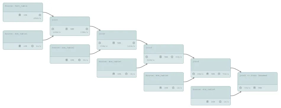
Together, this creates the following job graph which is quite similar to the SQL job above but does not need a Table conversion, nor a selection of according keys - this is built into the join function which uses alterations of the Fact class for each enrichment: Fact1, Fact2, …, Fact4, DenormalizedFact.
So far, so good - with and without object reuse, we are able to outperform Flink’s old planner by roughly 17%. The new Blink planner, however, is able to squeeze out a few more events per second after enabling object reuse. Actually, object reuse should not have any effect on our DataStream job since there are no chained operators; the 4% difference in the numbers below seem to come from normal fluctuations during the benchmark.
| Without Object Reuse | With Object Reuse | |
| SQL Join, Old Planner | 84,279 | 88,426 |
| SQL Join, Blink Planner | 89,048 | 136,710 |
| DataStream Join 1 | 99,025 | 103,102 |
Performance Analysis of the DataStream Job
I was actually expecting a bigger difference, so let us look at a profiler to see where CPU time is spent. You can use any profiler of your preference; I’m showing results from JMC 7 and ran LateralStreamJoin1 with Java 11 to get these results. As you can see, serialization work from DataOutputSerializer, StringValue, and reflective accesses outweigh the actual business logic, e.g. CopyOnWriteStateMap which is retrieving the matching dimensional data from the on-heap state or com.ververica.LateralStreamJoin1 for our actual code.
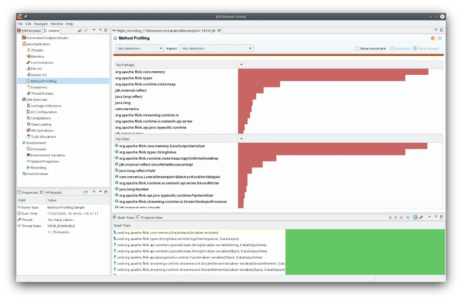
This is not really surprising since (de)serialization usually has a high overall cost and the presented job does not have (much) computation on its own - there is essentially only the one state access for each event from the fact stream. On the other hand, if we recall the job graph from above, there will be (de)serialization of the data from dim_table1 in each step: join1, join2, join3, join4, and join5 which is then the only/first place where it may actually be used. This is similar for the other dimensional tables and seems like something we could avoid.
Reducing the Serialization Overhead
In order to avoid the continuous (de)serialization of the same data over and over again, we could serialize it once at the source and then just pass it along until it is really needed, i.e. inside the join5 task. The quickest way of getting there, with our source generators, is to add a Map function that does this transformation:
class MapDimensionToBinary extends RichMapFunction<dimension, binarydimension=""> {
 private transient TypeSerializer dimSerializer;
 private transient DataOutputSerializer serializationBuffer;

 @Override
 public BinaryDimension map(Dimension value) throws Exception {
 return BinaryDimension.fromDimension(value, dimSerializer, serializationBuffer);
 }

 @Override
 public void open(Configuration parameters) throws Exception {
 serializationBuffer = new DataOutputSerializer(100);
 dimSerializer = TypeInformation.of(Dimension.class).createSerializer(getRuntimeContext().getExecutionConfig());
 }
}
BinaryDimension is a simple POJO with one long for the dimension key and a byte array for the serialized data. This is the object we would be passing around instead. Actually, if you look at the code of LateralStreamJoin2, you will see that we use Tuple2, …, Tuple5 instead (for simplicity) just as well as further (minor) improvements on the overhead since Tuple serialization is a bit faster than serializing POJOs. The job’s body thus only changes slightly by having these additional maps, a few changes to the participating types, and the deserialization after the final join.
StreamExecutionEnvironment env = StreamExecutionEnvironment.getExecutionEnvironment();

DataStream factTableSource = env
 .addSource(new FactTable(factTableRate, maxId))
 .name("fact_table");
DataStream dimTable1Source = env
 .addSource(new DimensionTable(dimTableRate, maxId))
 .name("dim_table1");
// ...

DataStream joinedStream =
 factTableSource
 .keyBy(x -> x.dim1)
 .connect(dimTable1Source.map(new MapDimensionToBinary()).keyBy(x -> x.id))
 .process(
 new AbstractFactDimTableJoin<fact, tuple2<fact,="" byte[]="">>() {
 @Override
 Tuple2<fact, byte[]=""> join(Fact value, BinaryDimension dim) {
 return Tuple2.of(value, dim.data);
 }
 })
 .name("join1").uid("join1")
// ...
 .keyBy(x -> x.f0.dim5)
 .connect(dimTable5Source.map(new MapDimensionToBinary()).keyBy(x -> x.id))
 .process(
 new AbstractFactDimTableJoin<tuple5<fact, byte[],="" byte[]="">, DenormalizedFact>() {
 private TypeSerializer dimSerializer;

 @Override
 DenormalizedFact join(Tuple5<fact, byte[],="" byte[]=""> value, BinaryDimension dim)
 throws IOException {
 DataInputDeserializer deserializerBuffer = new DataInputDeserializer();
 deserializerBuffer.setBuffer(value.f1);
 Dimension dim1 = dimSerializer.deserialize(deserializerBuffer);
 // ...
 return new DenormalizedFact(value.f0, dim1, dim2, dim3, dim4, dim5);
 }

 @Override
 public void open(Configuration parameters) throws Exception {
 dimSerializer =
 TypeInformation.of(Dimension.class)
 .createSerializer(getRuntimeContext().getExecutionConfig());
 }
 })
 .name("join5").uid("join5");

joinedStream.addSink(new DiscardingSink<>());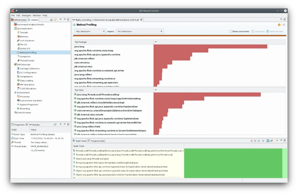
env.execute();</fact,></tuple5<fact,></fact,></fact,>The profiler snapshot from running this modified version of the job does indeed look different: while the top class ThreadLocal is still from (de)serialization (called StringValue.readString()), a considerable amount of CPU time goes into the actual logic, e.g. CopyOnWriteStateMap.
This additional efficiency is also reflected in the numbers of our benchmark. Without object reuse, the optimized version of the DataStream job is now roughly 70% faster than the SQL join using the Blink planner. Further enabling object reuse reduces the overhead of the new map operators as well as the final stage (writing to the sink) and provides a plus of 13%. The Blink planner, however, is able to gain a significantly larger increase by enabling object reuse (+54%).
In the end, our optimized DataStream job is thus 28% faster than the best we were able to achieve with SQL.
| Without Object Reuse | With Object Reuse | |
| SQL Join, Old Planner | 84,279 | 88,426 |
| SQL Join, Blink Planner | 89,048 | 136,710 |
| DataStream Join 1 | 99,025 | 103,102 |
| DataStream Join 2 | 154,402 | 174,766 |
Conclusion
Running this experiment shows an impressive performance of the Blink planner, when compared with the DataStream API. Something I was positively impressed by! In addition, future improvements to the Table API could actually reduce the gap a bit further, especially at places where the Table API needs to be bridged with the DataStream API. Using the DataStream API to improve the enrichment job’s performance further than the Blink planner requires careful considerations of the serialization stack and fine-tuning to the specific job at hand.
The presented technique basically relies on data staying in the serialized form as long as possible (when handed over via network) and only deserializing it when needed. This can probably be wrapped under some nice utility methods / base classes to improve the readability and usability of resulting code. However, when you look at the amount of code that was needed to make that optimization, you also have to take maintainability and development cost into account and decide about the trade-off, compared to the simplicity of SQL. More importantly, if the Blink planner introduces a specialized dimension join in the future, this optimization will be applied automatically under the hood without any change of the SQL query itself.