


In the previous article, we covered some aspects of time windows and time attributes that you should consider when planning your data collection strategy. This article will provide a more in-depth look at how to create a time window.
Note: A time window is the period of time over which data is collected. The length of the time window will depend on the type of data being collected and the purpose of the study. For example, if you are interested in studying the effects of a new product on consumer behavior, you would need to collect data over a longer period of time than if you were interested in studying the effects of a new marketing campaign on sales.
When selecting a time window for your case, you should consider the following attributes:
- Frequency of the data: If the data is collected daily, weekly, monthly, etc.
- Seasonality of the data: If the data is affected by seasonality (e.g. sales data is typically higher during the holiday season), you will need to take this into account when selecting a time window.
- Stability of the data: If the data is volatile (e.g. stock prices), you will need to take this into account when selecting a time window.
- Length of the time window: The length of the time window will depend on the type of data being collected and the purpose of the study.
Once you have considered the attributes of the data, you can select the most appropriate time window for your case.
How to create chained (event) time windows
This example will show you how to efficiently aggregate time series data on two different levels of granularity.
In this example, the source table (server_logs) is backed by the faker connector, which continuously generates rows in memory based on Java Faker expressions.
In the server_logs table, the average request size over one minute as well as five minute (event) windows will be computed. For this, you could run two queries, similar to the one in Aggregating Time Series Data from the Flink SQL cookbook. At the end of the page, you will find the script and the resulting JobGraph from this approach.
In the main part of the query, you will follow a slightly more efficient approach that chains the two aggregations: the one-minute aggregation output serves as the five-minute aggregation input.
Chained operators can be more efficient than using non-chained operators in terms of both latency and memory utilization.
Regarding latency, chained event time windows can reduce the overall processing time by allowing for multiple window operations to be performed in a single pass over the data. This can lead to a reduction in the amount of time it takes for the final results to be produced.
As for memory utilization, chained operators can also be more efficient because one UDF can call another UDF directly. Otherwise, each of them will run in its own threads.
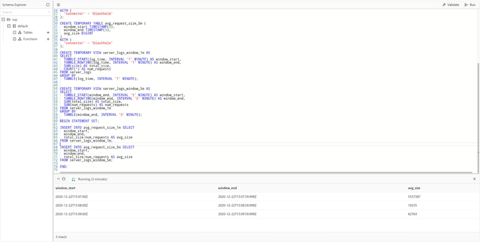
You will then use a Statements Set to write out the two result tables. To keep this example self-contained, you will use two tables of type blackhole (instead of kafka, filesystem, or any other connectors).
CREATE TEMPORARY TABLE server_logs (
    log_time TIMESTAMP(3),
    client_ip STRING,
    client_identity STRING,
    userid STRING,
    request_line STRING,
    status_code STRING,
    size INT,
    WATERMARK FOR log_time AS log_time - INTERVAL '15' SECONDS
) WITH (
  'connector' = 'faker',
  'fields.log_time.expression' =  '#{date.past ''15'',''5'',''SECONDS''}',
  'fields.client_ip.expression' = '#{Internet.publicIpV4Address}',
  'fields.client_identity.expression' =  '-',
  'fields.userid.expression' =  '-',
  'fields.request_line.expression' = '#{regexify ''(GET|POST|PUT|PATCH){1}''} #{regexify ''(/search\.html|/login\.html|/prod\.html|cart\.html|/order\.html){1}''} #{regexify ''(HTTP/1\.1|HTTP/2|/HTTP/1\.0){1}''}',
  'fields.status_code.expression' = '#{regexify ''(200|201|204|400|401|403|301){1}''}',
  'fields.size.expression' = '#{number.numberBetween ''100'',''10000000''}'
);

CREATE TEMPORARY TABLE avg_request_size_1m (
  window_start TIMESTAMP(3),
  window_end TIMESTAMP(3),
  avg_size BIGINT
)
WITH (
  'connector' = 'blackhole'
);

CREATE TEMPORARY TABLE avg_request_size_5m (
  window_start TIMESTAMP(3),
  window_end TIMESTAMP(3),
  avg_size BIGINT
)
WITH (
  'connector' = 'blackhole'
);

CREATE TEMPORARY VIEW server_logs_window_1m AS
SELECT
  TUMBLE_START(log_time, INTERVAL '1' MINUTE) AS window_start,
  TUMBLE_ROWTIME(log_time, INTERVAL '1' MINUTE) AS window_end,
  SUM(size) AS total_size,
  COUNT(*) AS num_requests
FROM server_logs
GROUP BY
  TUMBLE(log_time, INTERVAL '1' MINUTE);


CREATE TEMPORARY VIEW server_logs_window_5m AS
SELECT
  TUMBLE_START(window_end, INTERVAL '5' MINUTE) AS window_start,
  TUMBLE_ROWTIME(window_end, INTERVAL '5' MINUTE) AS window_end,
  SUM(total_size) AS total_size,
  SUM(num_requests) AS num_requests
FROM server_logs_window_1m
GROUP BY
  TUMBLE(window_end, INTERVAL '5' MINUTE);

BEGIN STATEMENT SET;

INSERT INTO avg_request_size_1m SELECT
  window_start,
  window_end,
  total_size/num_requests AS avg_size
FROM server_logs_window_1m;

INSERT INTO avg_request_size_5m SELECT
  window_start,
  window_end,
  total_size/num_requests AS avg_size
FROM server_logs_window_5m;

END;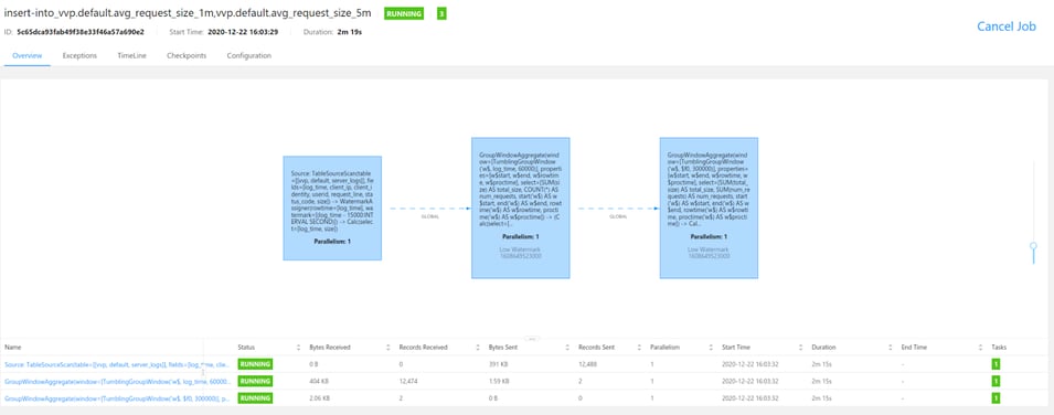
How to create non-chained windows
CREATE TEMPORARY TABLE server_logs (
    log_time TIMESTAMP(3),
    client_ip STRING,
    client_identity STRING,
    userid STRING,
    request_line STRING,
    status_code STRING,
    size INT,
    WATERMARK FOR log_time AS log_time - INTERVAL '15' SECONDS
) WITH (
  'connector' = 'faker',
  'fields.client_ip.expression' = '#{Internet.publicIpV4Address}',
  'fields.client_identity.expression' =  '-',
  'fields.userid.expression' =  '-',
  'fields.log_time.expression' =  '#{date.past ''15'',''5'',''SECONDS''}',
  'fields.request_line.expression' = '#{regexify ''(GET|POST|PUT|PATCH){1}''} #{regexify ''(/search\.html|/login\.html|/prod\.html|cart\.html|/order\.html){1}''} #{regexify ''(HTTP/1\.1|HTTP/2|/HTTP/1\.0){1}''}',
  'fields.status_code.expression' = '#{regexify ''(200|201|204|400|401|403|301){1}''}',
  'fields.size.expression' = '#{number.numberBetween ''100'',''10000000''}'
);

CREATE TEMPORARY TABLE avg_request_size_1m (
  window_start TIMESTAMP(3),
  window_end TIMESTAMP(3),
  avg_size BIGINT
)
WITH (
  'connector' = 'blackhole'
);

CREATE TEMPORARY TABLE avg_request_size_5m (
  window_start TIMESTAMP(3),
  window_end TIMESTAMP(3),
  avg_size BIGINT
)
WITH (
  'connector' = 'blackhole'
);

CREATE TEMPORARY VIEW server_logs_window_1m AS
SELECT
  TUMBLE_START(log_time, INTERVAL '1' MINUTE) AS window_start,
  TUMBLE_ROWTIME(log_time, INTERVAL '1' MINUTE) AS window_end,
  SUM(size) AS total_size,
  COUNT(*) AS num_requests
FROM server_logs
GROUP BY
  TUMBLE(log_time, INTERVAL '1' MINUTE);


CREATE TEMPORARY VIEW server_logs_window_5m AS
SELECT
  TUMBLE_START(log_time, INTERVAL '5' MINUTE) AS window_start,
  TUMBLE_ROWTIME(log_time, INTERVAL '5' MINUTE) AS window_end,
  SUM(size) AS total_size,
  COUNT(*) AS num_requests
FROM server_logs
GROUP BY
  TUMBLE(log_time, INTERVAL '5' MINUTE);

BEGIN STATEMENT SET;

INSERT INTO avg_request_size_1m SELECT
  window_start,
  window_end,
  total_size/num_requests AS avg_size
FROM server_logs_window_1m;

INSERT INTO avg_request_size_5m SELECT
  window_start,
  window_end,
  total_size/num_requests AS avg_size
FROM server_logs_window_5m;

END;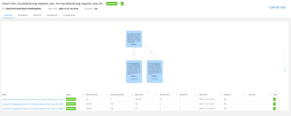
How to create hopping time windows
This example will show you how to calculate a moving average in real-time using a HOP window.
In this example, the source table (bids) is backed by the faker connector, which continuously generates rows in memory based on Java Faker expressions.
In one of our previous recipes, we've shown how you can aggregate time series datausing TUMBLE. To display every 30 seconds the moving average of bidding prices per currency per 1 minute, you will use the built-in HOPfunction.
The difference between a HOPand a TUMBLEfunction is that with a HOP you can "jump" forward in time. That's why you have to specify both the length of the window and the interval you want to jump forward. When using a HOPfunction, records can be assigned to multiple windows if the interval is smaller than the window length, like in this example. A tumbling window never overlaps and records will only belong to one window.
CREATE TABLE bids (
    bid_id STRING,
    currency_code STRING,
    bid_price DOUBLE,
    transaction_time TIMESTAMP(3),
    WATERMARK FOR transaction_time AS transaction_time - INTERVAL '5' SECONDS
) WITH (
  'connector' = 'faker',
  'fields.bid_id.expression' = '#{Internet.UUID}',
  'fields.currency_code.expression' = '#{regexify ''(EUR|USD|CNY)''}',
  'fields.bid_price.expression' = '#{Number.randomDouble ''2'',''1'',''150''}',
  'fields.transaction_time.expression' = '#{date.past ''30'',''SECONDS''}',
  'rows-per-second' = '100'
);

SELECT window_start, window_end, currency_code, ROUND(AVG(bid_price),2) AS MovingAverageBidPrice
  FROM TABLE(
    HOP(TABLE bids, DESCRIPTOR(transaction_time), INTERVAL '30' SECONDS, INTERVAL '1' MINUTE))
  GROUP BY window_start, window_end, currency_code;
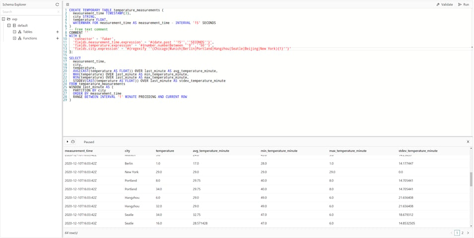
How to perform rolling aggregations on time series data
This example will show you how to calculate an aggregate or cumulative value based on a group of rows using an OVER window. A typical use case is rolling aggregations.
The source table (temperature_measurements) is backed by the faker connector, which continuously generates rows in memory based on Java Faker expressions.
OVER window aggregates compute an aggregated value for every input row over a range of ordered rows. In contrast to GROUP BY aggregates, OVER aggregates do not reduce the number of result rows to a single row for every group. Instead, OVER aggregates produce an aggregated value for every input row.
The order needs to be defined by a time attribute. The range of rows can be defined by a number of rows or a time interval.
In this example, you are trying to identify outliers in the temperature_measurements table. For this, you will use an OVER window to calculate, for each measurement, the maximum (MAX), minimum (MIN) and average (AVG) temperature across all measurements, as well as the standard deviation (STDDEV), for the same city over the previous minute.
CREATE TEMPORARY TABLE temperature_measurements (
  measurement_time TIMESTAMP(3),
  city STRING,
  temperature FLOAT,
  WATERMARK FOR measurement_time AS measurement_time - INTERVAL '15' SECONDS
)
WITH (
  'connector' = 'faker',
  'fields.measurement_time.expression' = '#{date.past ''15'',''SECONDS''}',
  'fields.temperature.expression' = '#{number.numberBetween ''0'',''50''}',
  'fields.city.expression' = '#{regexify ''(Chicago|Munich|Berlin|Portland|Hangzhou|Seatle|Beijing|New York){1}''}'
);

SELECT
  measurement_time,
  city,
  temperature,
  AVG(CAST(temperature AS FLOAT)) OVER last_minute AS avg_temperature_minute,
  MAX(temperature) OVER last_minute AS min_temperature_minute,
  MIN(temperature) OVER last_minute AS max_temperature_minute,
  STDDEV(CAST(temperature AS FLOAT)) OVER last_minute AS stdev_temperature_minute
FROM temperature_measurements
WINDOW last_minute AS (
  PARTITION BY city
  ORDER BY measurement_time
  RANGE BETWEEN INTERVAL '1' MINUTE PRECEDING AND CURRENT ROW
);
Conclusion
In this article, we have shown you a couple of Flink SQL examples for creating time windows, which can be useful in different situations. We have also shown you how to perform a chained windowing operation and a non-chained windowing operation.
We strongly encourage you to run these examples in Ververica Platform. Just follow these simple stepsto install the platform.
Follow us on Twitter to get updates on our next articles and/or to leave us feedback. :)
If you're interested in learning more about Flink SQL, we recommend the following resources:
You may also like

Your AI Coding Assistant Can't Touch Your Streaming Platform. Until Now

Zero Trust Theater and Why Most Streaming Platforms Are Pretenders

No False Trade-Offs: Introducing Ververica Bring Your Own Cloud for Microsoft Azure
