
This article is a follow-up post to the earlier published article about Computing recommendations at extreme scale with Apache Flink. We discuss how we implemented the alternating least squares (ALS) algorithm in Apache Flink, starting from a straightforward implementation of the algorithm, and moving to a blocked ALS implementation optimizing performance on the way. Similar observations have been made by others, and the final algorithm we arrive to is also the one implemented in Apache Spark's MLlib. Furthermore, we describe the improvements contributed to Flink in the wake of implementing ALS.
Prologue
Recommending the right products to users is the cornerstone for e-commerce and several internet companies. Examples of recommendations include recommending items at amazon.com, movies on netflix, songs at music services like Spotify, etc. Providing good recommendations improves the user experience and plays an important role in sales growth. There are two main approaches to recommendation: The first one is called content-based recommendation. Content-based methods try to create a feature vector for each item describing its properties. By knowing which items the user consumed before, we can look for other items which are similar with respect to some metric and recommend these items to the user. The drawback of this approach is that it is not always possible to find the right features to describe an item. The alternative approach is recommending items based on the past behaviour of a group of users. Depending on the preferences of users who behave similarly, one can make predictions about what other items a user might like. This approach is called collaborative filtering (CF). The advantage of CF is that it automatically detects relationships between users and interdependencies among items which are hard to capture by a content-based method. However, CF suffers from the cold start problem which arises if one introduces a new item for which no past behaviour exists. For these items it is hard to make predictions until some users have given initial feedback.
Latent factor models
One way to solve the problem of collaborative filtering are latent factor models. Latent factor models try to find a user-factor and item-factor vector $x_u, y_i \in \mathbb{R}^f$ for each user $u$ and item $i$ with $f$ being the number of latent factors such that the inner product calculates the prediction value $\hat{r}_{ui} = x_u^Ty_i$. The latent factors are the representation of user preferences and item characteristics in an abstract feature space. One could think of these variables as denoting the color, shape, price or the genre of an item. In general, the latent factors represent more abstract concepts which cannot be directly grasped.
Problem formulation
The following problem formulation is the summary of the work of Zhou et al. and Hu et al. Given the matrix of user-item ratings \(R=(r_{ui})\) with $u \in [1...n]$ and $i \in [1...m]$ where $r_{ui}$ represents the preference of user $u$ for item $i$ we can try to find the set of user- and item-factor vectors. It is noteworthy that $R$ is intrinsically sparse because usually a user has only given feedback to a subset of all items. Therefore, we will only consider the rated items of every user to measure the performance of our latent factors model. By finding a model whose predictions are close to the actual ratings, we hope to be able to make predictions for unrated items. Retrieving a suitable model boils down to a minimization problem of the root-mean-square error (RMSE) between existing ratings and their predicted values plus some regularization term to avoid overfitting: \[\min_{X,Y}\sum_{r_{ui}\text{ exists}}\left(r_{ui}-x_u^Ty_i\right)^2 + \lambda\left( \sum_{u}n_u||x_{u}||^2 + \sum_{i}n_i||y_{i}||^2\right)\] . $X=(x_1, \ldots, x_n)$ is the matrix of user-factor vectors and $Y=(y_1, \ldots, y_m)$ is the matrix of item-factor vectors. $n_u$ and $n_i$ denotes the number of existing ratings of user $u$ and item $i$, respectively. According to Zhou et al., this weighted-$\lambda$-regularization gives best empirical results. If we write this in matrix notation, then we easily see that we are actually looking for a low-rank matrix factorization of $R$ such that $R=X^TY$. By fixing one of the sought-after matrices we obtain a quadratic form which can be easily minimized with respect to the remaining matrix. If this step is applied alternately to both matrices we can guarantee that for each step we converge closer to the solution. This method is called alternating least squares (ALS). If we fix the item-factor matrix and solve for the user-factor matrix we obtain the following equation which we have to solve for each user-factor vector: \[x_{u} = \left(YS^uY^T + \lambda n_u I\right)^{-1}Yr_u^T\] with $r_u$ being the rating vector of user $u$ (the $u$th row vector of $R$) and $S^u \in \mathbb{R}^{m\times m}$ is the diagonal matrix where \[S^u_{ii}=\begin{cases} 1 & \text{if }r_{ui} \not = 0 \\ 0 & \text{else} \end{cases}\]. For the sake of simplicity we set $A_u = YS^uY^T + \lambda n_u I$ and $V_u = Yr_u^T$. The item-factor vectors can be calculated in a similar fashion: \[y_{i} = \left(XS^iX^T + \lambda n_i I\right)^{-1}Xr^i\] with $r^i$ being the rating vector of item $i$ ($i$th column vector of $R$) and $S^i \in \mathbb{R}^{n\times n}$ is the diagonal matrix where \[S^i_{uu} = \begin{cases} 1 & \text{if }r_{ui} \not = 0 \\ 0 & \text{else} \end{cases}\]. Again we can simplify the equation by $A_i = XS^iX^T + \lambda n_i I$ and $V_i = Xr^i$. Since we want to factorize rating matrices which are so big that they no longer fit into the main memory of a single machine, we have to solve the problem in parallel. Furthermore, the ALS computation is inherently iterative, consisting of a series of optimization steps. Apache Flink constitutes an excellent fit for this task, since it offers an expressive API combined with support for iterations. An in-depth description of Apache Flink's programming API can be found here. The rating matrix $R$ is sparse and consequently we should represent it as a set of tuples (rowIndex, columnIndex, entryValue). The resulting user-factor and item-factor matrices will be dense and we represent them as a set of column vectors (columnIndex, columnVector). If we want to distribute the rating and user/item matrices, we can simply use Flink’s DataSet, which is the basic abstraction to represent distributed data. Having defined the input and output types, we can look into the different implementations of ALS.
Act I: Naive ALS
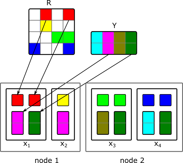
As a first implementation, we simply implemented the formulas of how to compute the user vectors from the item matrix and vice versa. For the first step, the item matrix is initialized randomly. In order to calculate a new user vector, we have to collect all item vectors for which the user has provided a rating. Having these vectors and the corresponding ratings, we can solve the equation which gives us the new user vector. Afterwards, the new DataSet of user vectors is used to compute the new item matrix. These two steps are executed iteratively to obtain the final solution. But how can we realize these operations with Flink? At first, we can observe that all item vectors are uniquely identified by their column indices. The same holds for the ratings which are identified by a pair of row and column indices (userID, itemID). We can combine the item vectors with their corresponding ratings by joining the item vectors with the ratings where the vector’s column index is equal to the column index of the rating. This join operation produces a tuple of user id $u$, the rating $r_{ui}$ and the corresponding item vector $y_{i}$. By grouping on the user id, we obtain all item vectors and the ratings for one user. Within the group reduce operation we can construct the matrix $A_u$ and the right-hand side $V_u$ from the item vectors. The solution to this equation system gives us the new $x_u$. The data partitioning of the group reduce operation is depicted in the figure below. Each user vector $x_u$ is calculated within its own parallel task.
The Flink code for one iteration step looks the following: [scala]// Generate tuples of items with their ratings val uVA = items.join(ratings).where(0).equalTo(1) { (item, ratingEntry) => { val Rating(uID, _, rating) = ratingEntry (uID, rating, item.factors) } } // Group item ratings per user and calculate new user-factor vector uVA.groupBy(0).reduceGroup { vectors => { var uID = -1 val matrix = FloatMatrix.zeros(factors, factors) val vector = FloatMatrix.zeros(factors) var n = 0 for((id, rating, v) <- vectors) { uID = id vector += rating * v matrix += outerProduct(v , v) n += 1 } for(idx <- 0 until factors) { matrix(idx, idx) += lambda * n } new Factors(uID, Solve(matrix, vector)) } }[/scala] This ALS implementation successfully computes the matrix factorization for all tested input sizes. However, it is far from optimal, since the algorithm creates for each user who rates an item $i$ a copy of the item vector $y_i$. If for example, several users which reside on one node have rated the same item, then each of them will receive their own copy of the item vector. Depending on the structure of the rating matrix, this can cause some serious network traffic which degrades the overall performance. A better solution which mitigates this problem will be presented in act III.
Act II: ALS with broadcasting
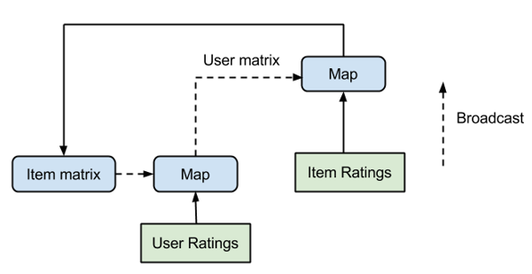
The naive ALS implementation had to calculate for each step which item vectors are needed to compute the next user vector. Depending on the density of the rating matrix $R$ it might be the case that almost all item vectors have to be transferred. In such a case, we could omit the expensive join and group reduce operations and simply broadcast the whole item matrix $Y$ to all cluster nodes. By grouping the ratings according to their user ids, we simply have to apply a map operation to the grouped user ratings. Within the map operation we have access to all of the broadcasted item vectors and the ratings of the respective user. Thus, we can easily calculate the new user vector. The corresponding data partitioning for the map operation which calculates the next user vectors is shown below. Each of the parallel tasks, responsible to calculate a single user vector $x_u$ only requires the respective user ratings. The necessary item vectors are accessed through the broadcasted item matrix.
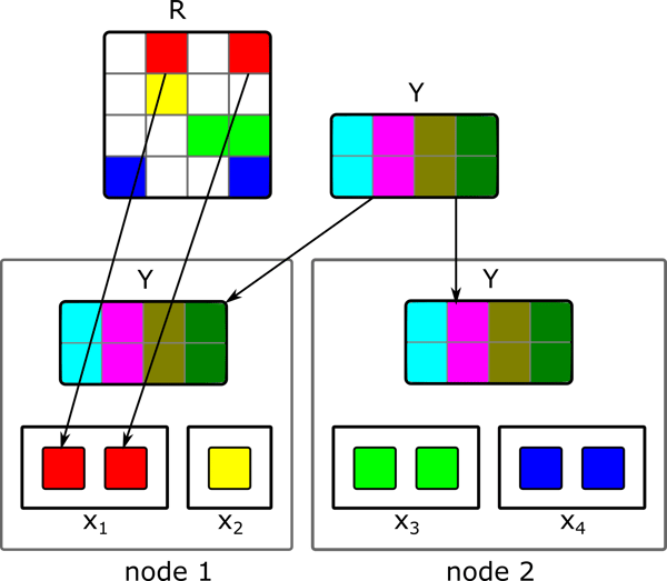
For the new item matrix we would do the same, only that we broadcast the new user matrix and group the ratings according to the item ids. The grouping of the ratings can be done outside of the iteration and thus will be calculated only once. Consequently, the final iteration step only consists of two map and two broadcast operations. The iteration is shown in the picture below.
To support the above presented algorithm efficiently we had to improve Flink’s broadcasting mechanism since it easily becomes the bottleneck of the implementation. The enhanced Flink version can share broadcast variables among multiple tasks running on the same machine. Sharing avoids having to keep for each task an individual copy of the broadcasted variable on the heap. This increases the memory efficiency significantly, especially if the broadcasted variables can grow up to several GBs of size.
Runtime comparison: Naive vs. Broadcast
In order to compare the performance of the broadcast variant to the naive ALS implementation, we measured the execution time for different input matrices. All experiments were run on Goolge Compute Engine where we used a cluster consisting of 40 medium instances (“n1-highmem-8”, 8 cores, 52 GB of memory). As input data, we generated random rating matrices of varying sizes and calculated 10 iterations of ALS with 50 latent factors. For each row of the random rating matrix a normal distributed number of non-zero entries was generated. We started with 400000 users and 50000 items where each user rated 200 items on average. We increased the size of the rating matrices up to 16 million users and 2 million items where each user rated 500 items on average. Thus, the largest rating matrix contained 8 billion ratings.
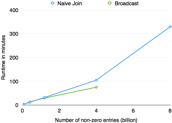
The simplification of the broadcast variant’s data flow leads to a significantly better runtime performance compared to the naive implementation. However, it comes at the price of degraded scalability. The broadcast variant only works if the complete item matrix can be kept in memory. Due to this limitation, the solution does not scale to data sizes which exceed the complete memory capacity. This disadvantage can be seen in the figure above. The factorization of our input matrices with more than 4 billion non-zero entries failed using the broadcast ALS version whereas the naive implementation successfully finished. The broadcast ALS implementation can be found here. The code for the naive join ALS implementation can be found here.
Act III: Blocked ALS
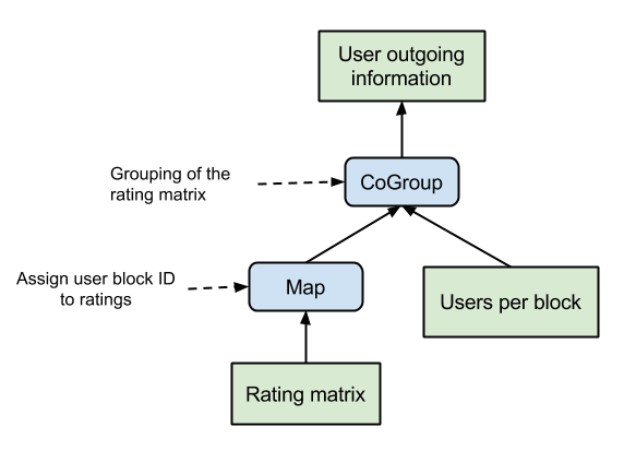
The main drawback of the naive implementation is that item vectors are sent to each user individually. For users residing on the same machine and having rated the same item this means that the item vector will be sent several times to this machine. That causes unnecessary network traffic and is especially grave since ALS is so communication intensive. The main idea to overcome this problem is to group the item vectors with respect to the users who are kept on the same machine. That way each item vector will be only sent at most once to each participating working machine. We achieve the user and item grouping by using blocks of users and items for our calculations instead of single users and items. These blocks will be henceforth called user and item blocks. Since we do not want to send each item block to all user blocks we first have to compute which item vectors of a given block has to be sent to which user block. With this outgoing information we can generate for each user block the partial item block update messages. In order to calculate the outgoing information we have to look for each user block $ub$ if there exists a user $u$ in block $ub$ who has rated a given item $i$ contained in block $ib$. If this is the case, then the block $ib$ has to send the item vector $y_i$ to the user block $ub$. This information can be calculated by grouping the rating matrix $R$ with respect to the item blocks and computing for each item to which user block it has to be sent. The corresponding data flow plan is given below.
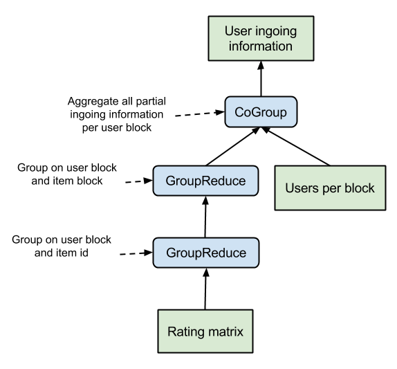
Additionally to the outgoing information, we also need the ingoing information to compute the user block updates out of the partial update messages. Since every item vector $i$ is only sent at most once to each user block and there might be several users in a block who have rated this item, we have to know who these users are and what their rating is. With this information, we can incrementally construct the matrices $A_u$ for all $u$ in a given block $b$ by adding the item vector $i$ only to those $A_u$ for which a rating $r_{ui}$ exists. That way, we do not have to keep all item vectors in memory and can instead work only on one partial update message at a time in a streaming-like fashion. The streaming aspect comes in handy for Flink’s runtime which natively supports pipelined operations and thus avoids to materialize intermediate results which can easily exceed the total memory size. The ingoing information are computed from the rating matrix $R$ by grouping it with respect to the user block and item. That way, we can compute for each user block $ub$ and item $i$ the set of users belonging to block $ub$ and having rated item $i$. By grouping these results according to the item block $ib$, we can compute the partial ingoing information for each pair of user and item blocks $(ub, ib)$. To finalize the ingoing information we simply have to aggregate all user-item block pairs with respect to the user block. The corresponding data flow is given below.
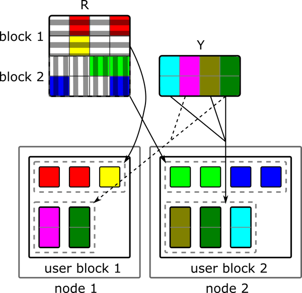
Having calculated these meta information and having blocked the user and item matrix, we can think about the actual ALS iteration step. The iteration step is in fact similar to the naive implementation only with the difference that we are operating on user and item blocks. At first, we have to generate the partial update messages for each user block. This can be done by joining the block item matrix with the outgoing item information. The outgoing information for the item block $ib$ contains the information to generate for each user block $ub$ a partial update message containing only the required item vectors from $ib$. The partial update messages are grouped according to their user block $ub$ and joined with the ingoing user information. The grouping and joining can be realized as a coGroup operation which avoids to explicitly construct an object containing all partial update messages. Instead we can exploit Flink’s streaming capabilities and process one partial update message after the other within the coGroup function. The coGroup function is responsible to construct the different $A_u$ matrices for each user $u$ in a user block. This can be done incrementally by adding the currently processed item vector $y_i$ from a partial update message to all $A_u$ and $V_u$ where the user $u$ has rated item $i$. The ingoing information contains this information and also the rating value. After having processed all partial update messages, the finished $A_u$ and $V_u$ can be used to calculate the new user vector $x_u$. The resulting data partitioning for the coGroup operation is depicted below. Ideally, we have only one user block per node so that the amount of redundantly sent data is minimized.
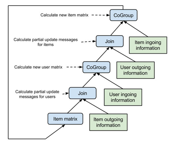
The same can be done to calculate the new item matrix based on the latest user matrix. We simply have to switch the outgoing item information with the outgoing user information, the ingoing user information with the ingoing item information and the item matrix with the user matrix to obtain the second half step of the ALS iteration. The complete data flow of the blocked ALS iteration is given in the figure below.
What are the secrets?
To support the above algorithm implementation efficiently, we relied heavily on Flink’s pipelined shuffles (that avoid materializing intermediate results) and its robust and efficient de-staging from in-memory to out-of-core processing. Furthermore, we found four new crucial features which we added to the system. While many data processing programs work on a large number of small records (billions of records of a few bytes to megabytes), this ALS implementation works on comparatively few records of large size (several 100 MB) due to the blocking. We added extra code paths to the internal sort algorithms of Flink to support memory efficient external sorting and merging of such large records. All code modifications mentioned in this blog post have been contributed back to the main code base of Flink. Building the matrix info blocks requires reduce functions to work on large groups of data. Flink supports streaming such groups through reduce functions to avoid collecting all objects, scaling to groups that are exceeding memory sizes. We added support to have the objects within the group stream sorted on additional fields, which is necessary to map the right partial update messages with the correct ingoing information. We tuned the network stack code that serializes records and breaks them into frames for network transfer, making sure that the subsystem does not hold onto many large objects concurrently. This increases Flink’s robustness, because Flink no longer runs easily out of memory when handling large records. Flink now supports user specified partitioners which allow to control how the data is distributed across the cluster. This is especially important if the user operates on few data items and wants to guarantee that it is evenly distributed. The custom partitioner is relevant if the number of user and item blocks is equal to the degree of parallelism. In such a scenario, the system should optimally distribute each block to a distinct processing task. The general-purpose partitioning algorithm cannot guarantee such a distribution but with a custom partitioner it is easily feasible. The code which implements the blocked ALS variant is based on the ALS implementation contained in Spark’s MLLib. The port contains modifications to optimize it for Flink’s runtime to be able to scale to really large input sizes. The blocked ALS code can be found here.
Runtime of blocked ALS implementation
In order to investigate the performance of Flink’s blocking ALS implementation, we ran a series of experiments again with the blocked ALS implementation on Google Compute Engine. This time, we used two cluster setups for the benchmarks. The first cluster setup was identical to the first experiments, consisting of 40 medium instances (“n1-highmem-8”, 8 cores, 52 GB of memory), and the second cluster setup consisted of 40 large instances (“n1-highmem-16”, 16 cores, 104 GB of memory). As input data, we generated random rating matrices of varying sizes and calculated 10 iterations of ALS with 50 latent factors. For each row of the random rating matrix a normal distributed number of non-zero entries was generated. We started with 400000 users and 50000 items where each user rated 200 items on average. We increased the size of the rating matrices up to 40 million users and 5 million items where each user rated 700 items on average. Thus, the largest rating matrix contained 28 billion ratings. This number of ratings poses a reasonable problem size as Netflix reported in 2012 to have 5 billion ratings.
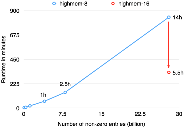
Both cluster setups use HDFS on disks for the rating matrix input, and Google Compute Engine's local SSDs for spilling intermediate results, sorts, and hash tables. The following figure shows how Flink’s performance scales with the data size using either 40 medium GCE machines (blue line), or 40 large GCE machines (red line). For a small dataset (4 million users, 500k items), Flink was able to run 10 iterations of ALS in just about 20 minutes. For the full dataset of 28 billion ratings (40 million users, 5 million items), Flink was able to finish the job in 5 hours and 30 minutes. This means a fresh recommendation model daily, even for an extremely large corpus of ratings. Note that while both the input data size (700 GB) and the sizes of the low-rank matrices (8.5 GB and 1.5 GB) are well below the aggregate memory of the cluster, the intermediate results (the vectors and factors exchanged between the user/item blocks) are several terabytes in size. In addition, two copies of the ratings matrix are cached - one partitioned by user, one partitioned by item. Many of the operations hence heavily rely on robust shuffling and out-of-core capabilities and use the local SSD storage.
Epilogue
In this report, we have seen that Flink can successfully factorize a matrix which has 28 billion non-zero entries and a size of 700 GB. The runtime of 5.5 h allows to calculate the factorization on a daily basis which can significantly improve the accuracy of recommendation systems. We implemented different versions of the popular ALS algorithm with weighted-$\lambda$-regularization. The blocked version exhibited the best performance with respect to scalability and runtime, because it notably reduced the amount of network traffic. However, the blocked ALS implementation posed some serious challenges for Flink to overcome first. To make this work, Flink’s capabilities to process really large records on the network- as well as on the operator-level were enhanced. Furthermore, the programmatic control of data distribution within the cluster was added, which now allows to realize even more efficient algorithm implementations with Flink.

You may also like

Preventing Blackouts: Real-Time Data Processing for Millisecond-Level Fault Handling

Real-Time Fraud Detection Using Complex Event Processing

Meet the Flink Forward Program Committee: A Q&A with Erik Schmiegelow