


Flink SQL is the most widely used relational API based on standard SQL. It provides unified batch processing and stream processing, which makes it easy to develop applications, and is already widely used for various use cases.
Unlike the DataStream API, which offers the primitives of stream processing in a relatively low-level imperative programming API, the Flink SQL API offers a relatively high-level declarative API. This means that a program written with the DataStream API will transform into an execution graph without any optimizations, whereas a program written with Flink SQL must undergo rich transformations before it becomes an execution graph. Currently, the SQL planner provides different optimization techniques and, thanks to that, these optimization methods will help you write efficient SQL code.
Six main factors that improve the performance for a Flink job are:
- Avoiding duplicate computing
- Reducing invalid data
- Solving data skew issues
- Improving operator throughput
- Reducing state access (streaming only)
- Reducing state size (streaming only)
In this post, we will introduce some SQL/operator improvements based on the above factors. We will also give you insights into Flink SQL including how it works under the hood, its workflows, best practices when writing your queries, and what is in store for the future.
Flink Operator Execution Mode
Before going into the optimization details, let's first gain a basic understanding of the execution mode of Flink operators and the optimization process of Flink SQL, which will help us better understand Flink SQL.
Flink is a unified batch and streaming processing engine, it provides a unified API, unified operator description, and unified execution framework. But the operator execution mode for batch and streaming is different.
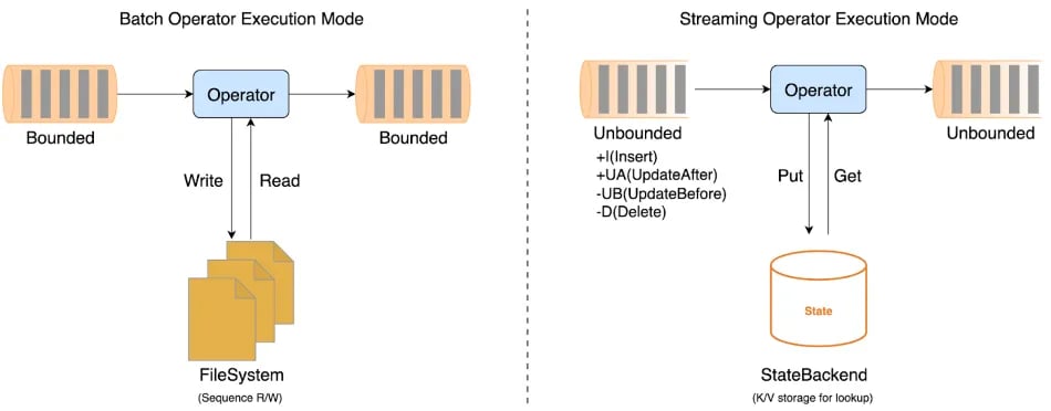
A batch operator will receive a bounded dataset as input and produce a bounded dataset as output. For the current implementation, the operator will process the all input data as a batch, and the data will be spilled to disk once the memory runs out. When designing and implementing batch operators, we should try to avoid disk access to improve performance.
A streaming operator, on the other hand, will take an unbounded dataset as input (also known as a Changelog) and output an unbounded dataset. Since the operator cannot buffer every piece of input data even with a disk, they will each be processed individually by the operator. The streaming operators must rely on State to store the intermediate computation results. When designing and implementing streaming operators, we should try to avoid state access to improve performance. The Changelog not only contains INSERT messages, but also retraction(UPDATE_BEFORE, UPDATE_AFTER, DELTE) messages. The matter of reducing the retraction messages also falls into the remit of streaming operators.
Flink SQL Workflow
In order to better help you understand how SQL code becomes an efficient Flink job, the following graph shows the internal Flink SQL workflow.
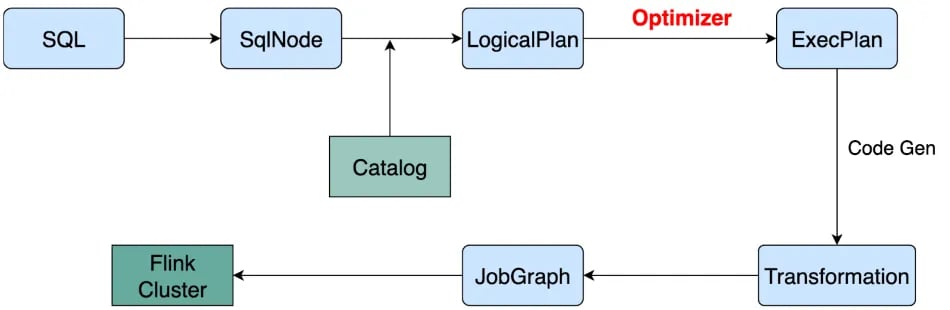
The transformation is deterministic from SQL text to LogicalPlan, and from ExecPlan to JobGraph. The optimizer is crucial even if there are numerous uncertainty transitions from LogicalPlan to ExecPlan. Now Let's take a rough look at the workflow of the optimizer.
Flink SQL Optimizer
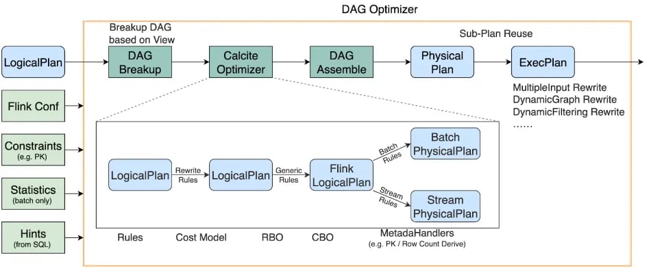
A Flink SQL job may contain multiple insert statements, which are parsed and converted into multiple logical trees, i.e. Directed Acyclic Graph (DAG). So, we call the optimizer a DAG optimizer. The DAG optimizer takes LogicalPlan, Flink Conf, Constraints and Statistics as input, and generates the optimized ExecPlan as output.
Flink uses Apache Calcite for relational algebra optimization, which can only accept a single logical expression tree. Therefore, after the optimizer receives a DAG, it will first break up the DAG into multiple logical expression trees based on the view, and then use Calcite to optimize the tree one by one. View-based breakup will reduce duplicate computing. After all the relational algebra expression trees are optimized, they will be reassembled into a DAG of the physical plan, and reduce repeated calculations through subgraph reuse technology to form an ExecPlan. Based on ExecPlan, we will make changes and write.
In the Calcite optimizer, we have implemented a large number of optimization rules and attribute derivation to help us generate the optimal execution plan.
Best Practices
Now, we will introduce some optimization options to improve the performance of Flink SQL jobs based on some high-frequency SQL cases used in our production.
Sub-Plan Reuse
Sub-Plan Reuse is mainly used for reducing duplicate computing, we will explain the details with the following simple example.
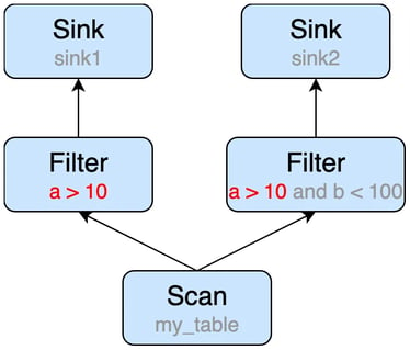
INSERT INTO sink1 SELECT * FROM my_table WHERE a > 10;
INSERT INTO sink2 SELECT * FROM my_table WHERE a > 10 AND b < 100;
The statements can be converted to the following execution plan, we can easily see that the Scan node will be executed twice, that is duplicate computing part (see the red dotted box).
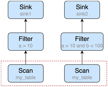
We can turn on Sub-plan Reuse by setting configuration table.optimizer.reuse-sub-plan-enabled=true (default is true), and the optimizer will automatically find and reuse the duplicate part in the DAG.
In the picture above, we can see that the scan operator is reused, but there is still a duplicate computing part (a > 10) after sub-plan reuse. It's very hard for the optimizer to find the duplicate computing expression in an operator, especially when the query is complex and various push down optimizations (e.g. filter push down, projection push down) are applied.
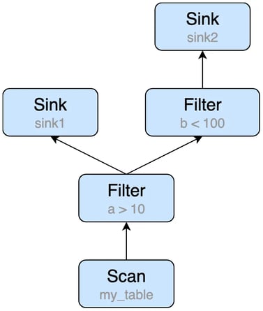
We recommend users to leverage View to solve the problem above. Views can not only improve the readability of the queries, but also help the optimizer find reusable parts. The query can be rewritten as the following:
CREATE TEMPORARY VIEW v1 SELECT * FROM my_table WHERE a > 10;
INSERT INTO sink1 SELECT * FROM v1;
INSERT INTO sink2 SELECT * FROM v1 WHERE b < 100;
The execution plan will be optimized as:
Fast Aggregation
Aggregate queries are widely used in Flink SQL. We will introduce some useful streaming aggregate optimization methods which could bring great improvement in some cases.
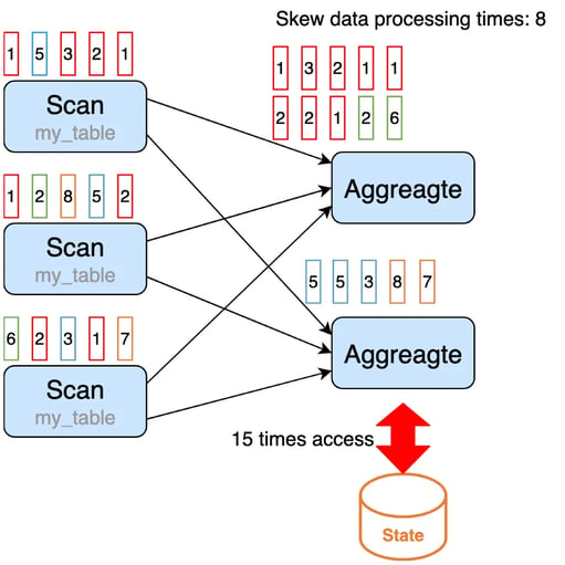
Streaming aggregation operator is a stateful operator, which uses state to store the intermediate aggregate results. By default, the streaming aggregation operators process input records one by one. When a record comes in, the operator will (1) read the accumulator from state, (2) accumulate/retract the record to the accumulator, (3) write the accumulator back to state. This processing pattern may cause performance problems of StateBackend, especially when State access is time-consuming and data skew exists after shuffling.
SELECT color, SUM(num) FROM my_table GROUP BY color;
In order to solve the above-mentioned problems, we have introduced various optimization options for different scenarios.
Note: The streaming aggregation optimizations mentioned in this section are all supported for Group Aggregations and Window TVF Aggregations now. We can also see the introduction in the Flink documentation.
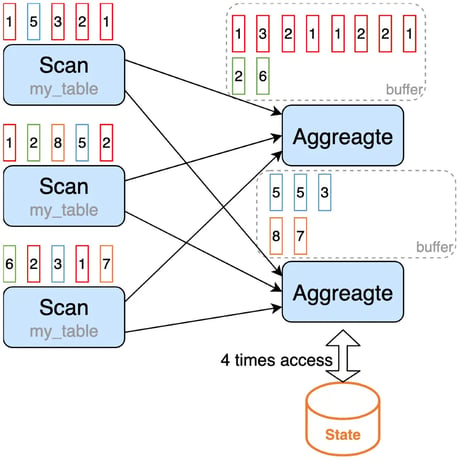
MiniBatch Aggregation
To reduce state access, we can introduce MiniBatch aggregation, which puts the input record into a buffer and triggers the aggregation operation after the buffer is full. The records with the same key in the buffer will be handled together, so only one operation per key to access state is needed.
MiniBatch Aggregation is disabled by default, we should set the following options to enable it.
table.exec.mini-batch.enabled: true // enable mini-batch
table.exec.mini-batch.allow-latency: 5s // put the records into a buffer within 5 seconds
MiniBatch can significantly reduce the state access and get better throughput. However, this will increase latency because the operator starts processing the records until the buffer is full instead of processing them in an instant. It is a trade-off between throughput and latency. Another benefit of MiniBatch is that the aggregation operator will output fewer records, especially in scenarios where there are retraction messages and the processing performance of downstream operators is insufficient.
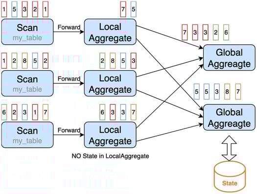
Local/Global Aggregation
In the example above, the data is skewed after shuffling, the first aggregate operator instance will process more data than other instances. This may cause performance problems.
To solve this, we can introduce Local/Global aggregation, which divides the aggregation into two stages, that is doing local aggregation in upstream (before shuffling) firstly, and followed by global aggregation in downstream (after shuffling). The local aggregation is chained with its upstream operator, this could avoid data skew caused by shuffling.
Local/Global Aggregation is disabled by default, we can set the following options to enable it, while making sure that all aggregate functions in a query must implement the merge method.
table.exec.mini-batch.enabled: true // enable mini-batch
table.exec.mini-batch.allow-latency: 5s // do a local aggregation within 5 seconds
table.optimizer.agg-phase-strategy: TWO_PHASE/AUTO // enable two phase aggregation
Local/Global Aggregation cannot solve the data-skew issues for distinct aggregation if the distinct key is sparse, the following example illustrates this problem.
SELECT color, COUNT(DISTINCT id) FROM my_table GROUP BY color;
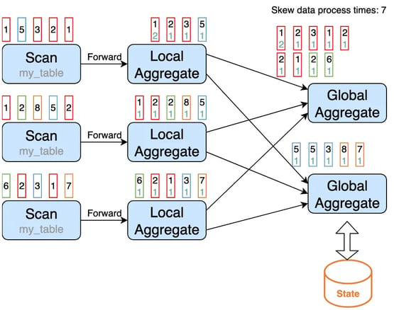
To solve this, we can introduce partial/final aggregation, which splits the distinct aggregation into two levels. The first aggregation (called partial aggregation) is shuffled by group key and an additional bucket key, which is HASH_CODE(distinct_key) % BUCKET_NUM. The second aggregation (called final aggregation) is shuffled by group key, and uses SUM to aggregate COUNT DISTINCT values from different buckets. The capacity to scale the job to solve data skew in distinct aggregations depends on the bucket key.
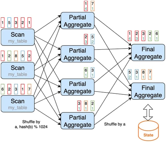
We can manually rewrite the above query into the following to enable partial/final aggregation.
SELECT color, SUM(cnt) FROM (
  SELECT color, COUNT(DISTINCT id) as cnt
  FROM my_table
  GROUP BY color, MOD(HASH_CODE(id), 1024)
) GROUP BY color;
Or, we can set the following options to enable it, while making sure that all aggregate functions in a query must be built-in aggregation functions and be splittable, e.g. AVG, SUM, COUNT, MAX, MIN.
table.optimizer.distinct-agg.split.enabled: true // enable partial/final aggregation
table.optimizer.distinct-agg.split.bucket-num: 1024 // bucket number
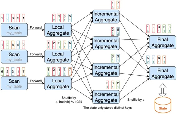
Incremental Aggregation
The state for partial aggregation may be very large if the distinct key is very sparse. We can introduce incremental aggregation to reduce the state size of partial aggregation. The state of incremental aggregation only stores the distinct keys, the aggregation function values will be stored in final aggregation.
To enable incremental aggregation, we should set the following options, and also make sure the query supports MiniBatch optimization, Local/Global optimization and Partial/Final optimization at the same time.
table.exec.mini-batch.enabled: true // enable mini-batch
table.exec.mini-batch.allow-latency: 5s // do a local aggregation within 5 seconds
table.optimizer.agg-phase-strategy: TWO_PHASE/AUTO // enable two phase aggreation
table.optimizer.distinct-agg.split.enabled: true // enable partail/final aggregation
table.optimizer.distinct-agg.split.bucket-num: 1024 // bucket number
table.optimizer.incremental-agg-enabled: true // enable incremental agg, default is true
Distinct Aggregate Function with FILTER
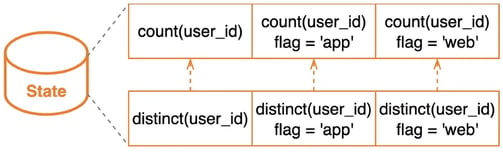
In some cases, a query calculates distinct results based on the same value but different dimensions. Such as: a user wants to calculate the number of UV (unique visitor) from different dimensions, e.g. UV from App, UV from Web and the total UV. Many users choose CASE WHEN to support this, for example:
SELECT
day,
COUNT(DISTINCT user_id) AS total_uv,
COUNT(DISTINCT CASE WHEN flag = 'app' THEN user_id ELSE NULL END) AS app_uv,
COUNT(DISTINCT CASE WHEN flag = 'web' THEN user_id ELSE NULL END) AS web_uv
FROM my_table
GROUP BY day;
For the query above, the state corresponding to the same function with the same distinct field is stored independently in an aggregation operator. The state structure is shown in the figure below.
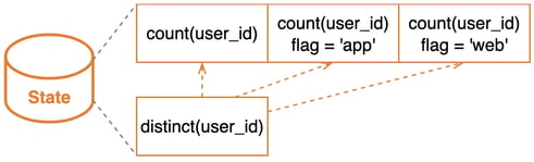
We recommend using FILTER syntax instead of CASE WHEN to let the planner do more optimizations to reduce the state size. Besides, FILTER is more compliant with the SQL standard.
SELECT
day,
COUNT(DISTINCT user_id) AS total_uv,
COUNT(DISTINCT) FILTER (WHERE flag = 'app') AS app_uv,
COUNT(DISTINCT) FILTER (WHERE flag = 'web') AS web_uv
FROM my_table
GROUP BY day;
After the query is rewritten, the state corresponding to the same function with the same different fields will be stored and shared in an aggregate operator. The new state structure can be improved as follows.
Fast Join
Join queries are widely used in FLINK SQL. There are different types of joins in streaming queries, the join in batch processing is called regular join in stream processing. Regular join is the most generic type of join in which any new record, or changes to either side of the join, are visible and affect the entirety of the join result. The state of regular join keeps both sides of the join input forever. The required state for computing the query result might grow infinitely depending on the number of distinct input rows of all input tables and intermediate join results. Reducing the state size is the key to optimize regular join performance.
There are three suggestions to reduce the state size of regular join:
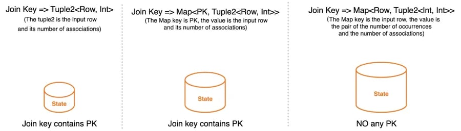
- Please make sure the join key contains the primary key or the join input has the primary key. In the following figure, we can see the state size for each case.
- Only keep the necessary fields before join operation.
- In addition to regular join, Flink also provides other types of joins, such as: Lookup Join, Temporal Join, Interval Join, Window Join If you can make some trade-offs in business, join can be rewritten as other joins.
SELECT *
FROM my_table1 t1
JOIN my_table2 t2
ON t1.a = t2.c;
- Regular joins are rewritten as temporal joins. Temporal joins allow joining against a versioned table, records from the probe side are always joined with the build side’s version at the time specified by the time attribute. As time passes, versions of the record that are no longer needed (for the given primary key) will be removed from the state. So the state size of temporal joins is less than regular joins.
SELECT *
FROM my_table1 t1
JOIN my_table2 FOR SYSTEM_TIME AS OF t1.row_time t2
ON t1.a = t2.c;
- Regular joins are rewritten as lookup joins. Lookup joins are typically used to enrich or filter the main-stream (a.k.a probe side) data. Records from the probe side are always joined with the latest version in the lookup source connector. Different from other joins, only the probe side can trigger the join operation, and the build side will not trigger even if it receives a new record. So lookup joins don't need state to store the input records. Please see "Fast Lookup Join" for more optimization.
SELECT *
FROM my_table1 t1
JOIN my_table2 FOR SYSTEM_TIME AS OF t1.proctime AS t2
ON t1.a = t2.c;
- Regular joins are rewritten as Interval joins. Interval joins allow joining the elements of two streams that share a common key and are within a time range. Interval joins only support append-only tables with time attributes. Since time attributes are quasi-monotonic increasing, Flink can remove old values from its state without affecting the correctness of the result. So the state size of interval joins is less than regular joins.
SELECT *
FROM my_table1 t1
JOIN my_table2 t2
ON t1.a = t2.c AND t1.row_time BETWEEN t2.row_time - INTERVAL '10' MINUTE AND t2.row_time;
- Regular joins are rewritten as window joins. Windows joins allow joining the elements of two streams that share a common key and are in the same window. Unlike other joins on continuous tables, window join does not emit intermediate results but only emits final results at the end of the window. Moreover, window join purges all intermediate states when no longer needed. So the state size of window joins is also less than regular joins.
SELECT * FROM (
 SELECT * FROM TABLE(TUMBLE(TABLE my_table1, å
  DESCRIPTOR(row_time), INTERVAL '10' MINUTES))
) t1 JOIN (
 SELECT * FROM TABLE(TUMBLE(TABLE my_table2,
  DESCRIPTOR(row_time), INTERVAL '10' MINUTES))
) t2
ON t1.window_start = t2.window_start
AND t1.window_end = t2.window_end
AND t1.a = t2.c;
Fast Lookup Join
Compared with other types of join, lookup join is the most widely used in production, so here is a further introduction to its optimization. We provide multiple optimization options to improve throughput:
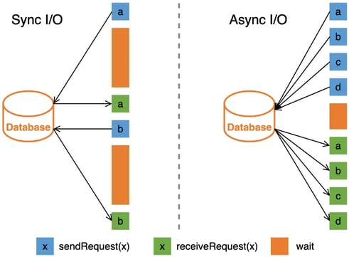
- Use Sync and Async Lookup Function
Lookup function can support both synchronous (sync) mode and asynchronous (async), their operating mechanism is as follows, and we can see the asynchronous mode has higher throughput.
If the connector has async lookup capability, we can use LOOKUP hints to suggest the planner to use the async lookup function.
-- use async mode
SELECT /*+ LOOKUP('table'='my_table2', 'async'='true') */ *
FROM my_table1 AS t1 JOIN my_table2
FOR SYSTEM_TIME AS of t1.proctime AS t2 ON t1.a = t2.c;

-- use sync mode
SELECT /*+ LOOKUP('table'='my_table2', 'async'='false') */ *
FROM my_table1 AS t1 JOIN my_table2
FOR SYSTEM_TIME AS of t1.proctime AS t2 ON t1.a = t2.c;
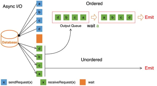
- Use ordered mode and unordered mode for async output mode.
In async mode, there are two modes to control in which order the resulting records are emitted:
- Ordered: Result records are emitted in the same order as the asynchronous requests are triggered (the order of the operators input records).
- Unordered: Result records are emitted as soon as the asynchronous request finishes. The order of the records in the stream may be different after the async I/O operator than before. It has higher throughput than ordered mode.
We can also use LOOKUP hints to suggest the planner to use the unordered mode.
-- use unordered mode
SELECT /*+ LOOKUP('table'='my_table2', 'async'='true')
     'output-mode'='allow_unordered', 'capacity'='100',
     'timeout'='180s') */ *
FROM my_table1 AS t1 JOIN my_table2
FOR SYSTEM_TIME AS of t1.proctime AS t2 ON t1.a = t2.c;

-- use ordered mode
SELECT /*+ LOOKUP('table'='my_table2', 'async'='true')
     'output-mode'='ordered', 'capacity'='100',
     'timeout'='180s') */ *
FROM my_table1 AS t1 JOIN my_table2
FOR SYSTEM_TIME AS of t1.proctime AS t2 ON t1.a = t2.c;
- Use CACHE
Caching is a common solution to reduce I/O and speed up lookup performance. Flink provides three caching strategies, FULL caching for small dataset, PARTIAL caching for large dataset, and NONE caching to disable it. We can also use rich options to control caching behavior.
Fast Deduplication
The upstream jobs may not have end-to-end exactly-once, which will result in data duplication in the source table. So we often encounter the requirement to keep the first or last row. Flink SQL does not provide deduplication syntax. In previous versions, Flink used an aggregation query with FIRST_VALUE to find the first row for a key or with LAST_VALUE to find the last row for a key.
-- find the first row per key
SELECT key, FIRST_VALUE(a), FIRST_VALUE(b) FROM my_table GROUP BY key;

-- find the last row per key
SELECT key, LAST_VALUE(a), LAST_VALUE(b) FROM my_table GROUP BY key;
From the "Fast Aggregation" section, we can see the aggregation operator will store a complete row for each key, which will cause the large state size. The FIRST_VALUE and LAST_VALUE aggregate function will ignore null values, which will cause wrong results if some columns have null values.
Now, Flink SQL uses ROW_NUMBER() to remove duplicates, just like the way of the Top-N query.
-- find the first row per key
SELECT a, b, c FROM (
 SELECT a, b, c,
  ROW_NUMBER() OVER (PARTITION BY a ORDER BY time_attr ASC) AS rn
  FROM my_table)
WHERE rn = 1;

-- find the last row per key
SELECT a, b, c FROM (
 SELECT a, b, c,
  ROW_NUMBER() OVER (PARTITION BY a ORDER BY time_attr DESC) AS rn
  FROM my_table)
WHERE rn = 1;
For the first row, the operator only needs to store the first row of each key, and for the last row, the operator only needs to store the last row for each key. At the same time, there is no problem with wrong results.
Fast TOP-N
Top-N (a.k.a Rank) queries are always used to get the N smallest or largest values. Flink SQL does not provide Top-N specific syntax but uses the combination of an OVER window clause and a filter condition to express a Top-N query. Now Flink SQL provides 3 kinds of rank algorithms with their performance decreasing sequentially.
- AppendRank: Only this algorithm is supported for insert-only changes input. The state of the rank operator stores the N smallest or largest records for each key.
- UpdateFastRank: Only this algorithm is supported iff the following requirements are met:
- The input produces update changes,
- The upsert key of input must contain the partition key for the over query,
- The order-by fields in the OVER query are monotonic, and the monotonic direction is opposite to the order-by direction.
The following query can be converted to the UpdateFastRank operator.
SELECT a, b, c FROM (
 SELECT a, b, c,
  ROW_NUMBER() OVER (
   -- The upsert key from upstream contains partition key
   PARTITION BY a, b
   -- c is monotonically increasing, while the order-by
   -- direction is monotonically decreasing
   ORDER BY c DESC) AS rn
  FROM (
  SELECT a, b,
    -- Declare the argument of sum to be a positive number,
    -- So that the result of sum is monotonically increasing
   SUM(c) FILTER (WHERE c >= 0) AS c
   FROM my_table
   -- Produce upsert stream, the upsert key is a, b
    GROUP BY a, b))
WHERE rn < 10;
The state of UpdateFastRank stores a map, its key is order key and its value is the record and the order number. The state size is greater than AppendRank, but less than RetractRank.
- RetractRank: This algorithm is supported for all queries. The state will store all the input data, so the state size may be very large. For optimization, the planner will try best to convert a given query into an AppendRank first, and then UpdateFastRank.
In addition to modifying the query to meet different rank algorithms, there are also some other optimization techniques to reduce state size or speed up state access.
- Do not output a rank number. This significantly reduces the amount of data that is to be written to the result table. The results can be sorted when they are finally displayed in the frontend.
- Increase the cache size of the rank operator. Rank operator provides a cache mechanism to reduce state access. The following formula is used to calculate the cache hit ratio:
cache_hit = cache_size * parallelism / top_n_num / partition_key_num
The state size is configured by table.exec.rank.topn-cache-size, the default value is 10000. If the parallelism is 50 and the top-n number is 100 and the number of partition key is 100000, we can get the cache hit is 10000 * 50 / 100 / 100000 = 5%. In this case, 95% requests will access the state backend directly. If we increase the cache size to 200000, the cache hit will be 200000 * 50 / 100 / 100000 = 100%, which indicates no request will access the state backend.
Please note that heap memory of the task manager needs to increase with the increase of cache size, otherwise OOM exceptions may occur.
Include a time field in the PARTITION BY clause. By default, the data in state has nothing to do with time, and the state of the rank operator cannot be cleaned, otherwise it will produce the wrong results. If we can add a time field in the PARTITION BY clause, we can also configure the time-to-live (TTL) to clean the outdated state data. Such as, we add the Day field to PARTITION BY and configure the TTL as 1.5 days.
Efficient User Defined Connector
Flink SQL provides multiple interfaces to optimize user defined source connectors. You should implement the following interfaces as needed:
- SupportsFilterPushDown: The planner will push the filters into the table source connector to avoid reading invalid data and reduce scan I/O.
- SupportsProjectionPushDown: The planner will push the needed fields into the table source connector to avoid reading invalid columns and reduce scan I/O.
- SupportsPartitionPushDown: The planner will push the needed partition list into the table source connector to avoid reading invalid partitions and reduce scan I/O.
- SupportsDynamicFiltering: The planner will push the dynamic filtering information into the table source connector to avoid reading invalid partitions and reduce scan I/O. Different from SupportsPartitionPushDown, filtering invalid partitions will happen at runtime rather than at the static planning stage.
- SupportsLimitPushDown: The planner will push the limit information into the table source connector to avoid reading redundant data, only the number of limit records will be read for each source instance.
- SupportsAggregatePushDown: The planner will push the aggregate functions into the table source connector to reduce scan I/O.
- SupportsStatisticReport: The planner could get statistics from the table source connector, and can generate a better execution plan.
Use Hints Well
Flink SQL supports changing execution behavior via hints. There are two kinds of hints:
- Table Hints: Table Hints (a.k.a Dynamic table options) allows to specify or override table options dynamically. For example, we can use /*+ OPTIONS('lookup.cache'='FULL') */ to change the cache strategy of the lookup table.
- Query Hints: Query hints can be used to suggest the optimizer to affect query execution plans within a specified query scope. LOOKUP hint is used to change lookup join operator behavior. For example, use /*+ LOOKUP('table'='my_table2', 'async'= 'true') */ to enable the async lookup function. BROADCAST, SHUFFLE_HASH, SHUFFLE_MERGE and NEST_LOOP hints are used to choose batch join strategy. For example, use /*+ BROADCAST(t1)*/ to suggest the optimizer chooses Broadcast Hash Join.
Future Developments
In the future, we will continue to improve the planner and focus on three areas:
- Deeper optimization: We will continue to work hard on the depth of optimization, such as incremental join, multiple joins.
- Richer optimization: We will closely combine more business scenarios for optimization.
- Smarter optimization: We will combine dynamic information at runtime for optimization, such as dynamic planning optimization.
You may also like

Zero Trust Theater and Why Most Streaming Platforms Are Pretenders

No False Trade-Offs: Introducing Ververica Bring Your Own Cloud for Microsoft Azure

Data Sovereignty Is Existential Most Platforms Treat It Like a Feature
